Better edges
Different hybrid edge styles
We can use the style and curved options to visualize hybrid edges in various ways. We will see examples later when hybrid edges are drawn straight with curved=:none, or only minor hybrid edges are curved with curved=:minor. By default curved=:both so both minor and major edges are curved.
- The default
style = :majortreehas the advantage of drawing each minor edge as a single segment, but the disadvantage of being unable to draw it proportional to the edge length (because the segment connects its 2 nodes, whose placements are dictated by the other edges). - The
:fulltreestyle draws each minor edge as 2 segments: one straight whose length can represent the edge length, and another segment (diagonal straight or curved) connecting to the hybrid child.
using RCall # to add annotations to the R-based plot
plot(net, style=:majortree); # default
R"mtext"("style = :majortree", side=1, line=-2);
plot(net, style=:fulltree);
R"mtext"("style = :fulltree", side=1, line=-2);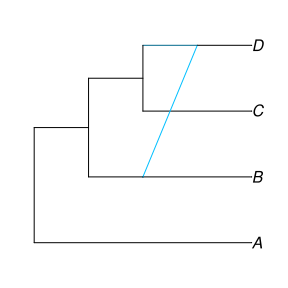
Using edge lengths
We can use useedgelength=true to draw a plot that uses the network's edge lengths to determine the lengths of the lines. For this, we'll use a network that has branch lengths:
net = readnewick("(A:3.3,((B:1.5,#H1:0.5):1.5,((C:1)#H1:1.8,D:1.1):.2):0.3);")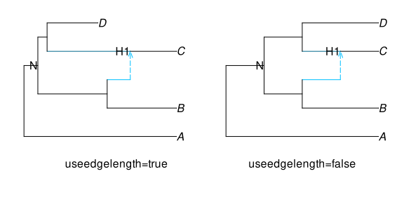
We used a DataFrame (not shown) to add the label "N". For more on this, see the section on Adding labels.
If branch lengths represent time, D could represent a fossil, or a virus strain sequenced a year before the others. Seeing this visually is the advantage of useedgelength=true.
This network happens to be time consistent, because the distance along the time (x) axis from node N to the hybrid node is the same both ways: the "upper" path has length 0.2 + 1.8 = 2, which is the same along the "lower" path, 1.5 + 0.5 = 2. We used option showedgelength=true to annotate the edges with their length.
A network is time-consistent if all the paths between 2 given nodes all have the same length. Time inconsistency can occur when branch lengths are not measured in calendar time, such as if branch lengths are in substitutions per site (some paths might evolve with more substitutions than others), or in number of generations (some lineages might have 1 generation per year, others more or fewer generations per year), or in coalescent units (number of generations / effective population size).
A time-consistent network may be ultrametric (the distance between the root and the tips is the same across all tips), or not like the network above.
Time-inconsistent networks like these ones below might cause confusion. Below we use the :fulltree style for the minor hybrid edges to have a straight segment showing (proportional to) their length.
net1 = readnewick("(A:3.3,((B:1.5,#H1:1.2):1.5,((C:1.8)#H1:1,D:1.1):.2):0.3);");
net2 = readnewick("(A:3.3,((B:1.5,#H1:0.2):1.5,((C:1)#H1:1.8,D:1.1):.2):0.3);");
plot(net1, style=:fulltree, curved=:minor,
     useedgelength=true, showedgelength=true);
plot(net2, style=:fulltree, curved=:minor,
     useedgelength=true, showedgelength=true);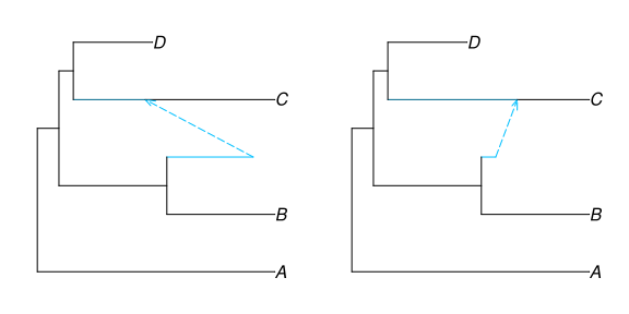
The default style=:majortree simplifies the visualization, as it does not visually represent minor edge lengths. Because of this, the option showedgelength=true to annotate each edge with its length gives us the information anyway.
plot(net1, useedgelength=true, showedgelength=true);
plot(net2, useedgelength=true, showedgelength=true);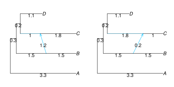
Varying edge widths
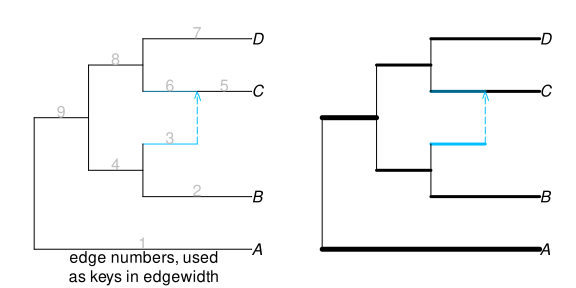
We can vary edge widths to show population sizes for example. First we need to map each edge number to the desired width for that edge. We do this with a dictionary.
julia> using RCall # to send any command to R, to modify the plotjulia> R"par"(mar=[.1,0,0,0]); R"layout"([1 2]);julia> plot(net1, showedgenumber=true);julia> R"mtext"("edge numbers, used\nas keys in edgewidth", side=1, line=-1);julia> # below: population sizes on the log scale log_populationsize = Dict(e.number => log10(1_000) for e in net1.edge);julia> log_populationsize[9] = log10(100_000); # larger populations on edge 9julia> log_populationsize[1] = log10(100_000); # and on edge 1julia> log_populationsizeDict{Int64, Float64} with 9 entries: 5 => 3.0 4 => 3.0 6 => 3.0 7 => 3.0 2 => 3.0 9 => 5.0 8 => 3.0 3 => 3.0 1 => 5.0julia> plot(net1, edgewidth=log_populationsize);
Customization
Check out the list of plot options.
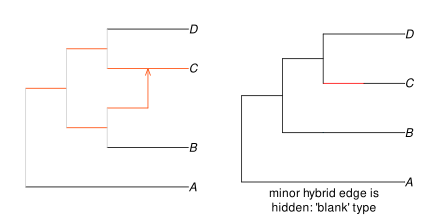
In the example below, we first highlight in orange the edges on the 2 paths from the root to C. Then we change the type of the minor edge (to hide it).
julia> ecols = Dict(i => "black" for i in 1:9); # make all blackjulia> for i in [9,8,6,5, 4,3] # except for edges ancestral to C ecols[i] = "orangered" endjulia> ecolsDict{Int64, String} with 9 entries: 5 => "orangered" 4 => "orangered" 6 => "orangered" 7 => "black" 2 => "black" 9 => "orangered" 8 => "orangered" 3 => "orangered" 1 => "black"
plot(net1, edgecolor=ecols, defaultedgecolor="grey80",
     minorlinetype="solid");
plot(net1, majorhybridedgecolor="red", defaultedgecolor="grey80",
     minorlinetype="blank", curved=:minor); # make minor edges (arrows) of type 'blank'