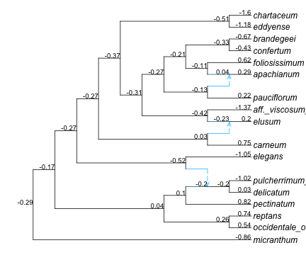
From the intercept coefficient we get a prediction at the root (-0.293 on the log scale) but that’s it.
predict ancestral states
This is typically called “ancestral state reconstruction” but prediction seems a more accurate term. This technique estimates the mean of nodes in the network: ancestral or extant species, conditional on the data. It’s important to look at prediction intervals, not just a “point” estimate.
asr =ancestralreconstruction(fit)asr_pred =predict(asr) # predictions at all nodes
39×2 DataFrame
14 rows omitted
Row
nodenumber
prediction
Int64
Float64
1
-5
0.257485
2
-8
-0.201828
3
7
-0.198663
4
-6
0.100981
5
-4
0.0403307
6
-10
-0.51602
7
-12
0.0315958
8
10
-0.230829
9
-15
-0.421436
10
-18
-0.130946
11
14
0.0351552
12
-20
-0.111023
13
-22
-0.326108
⋮
⋮
⋮
28
17
-0.427755
29
5
0.0306633
30
19
-1.17776
31
8
-1.05488
32
11
0.204422
33
16
0.621485
34
1
-0.863985
35
2
0.542107
36
13
0.220229
37
4
0.81878
38
6
-1.02358
39
3
0.744526
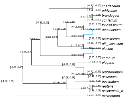
This output is somewhat cryptic though, because each row refers to a node number and it’s unclear which are tips, which are internal nodes, and which node has what number. We can also get prediction intervals (sometimes called confidence intervals) but with the same cryptic ordering of nodes:
asr_pred_int =predict(asr, interval =:prediction)
39×4 DataFrame
14 rows omitted
Row
nodenumber
prediction
lower
upper
Int64
Float64
Float64
Float64
1
-5
0.257485
-0.522481
1.03745
2
-8
-0.201828
-0.797811
0.394156
3
7
-0.198663
-0.790369
0.393042
4
-6
0.100981
-0.691258
0.893219
5
-4
0.0403307
-0.657145
0.737806
6
-10
-0.51602
-1.31902
0.286976
7
-12
0.0315958
-0.828791
0.891983
8
10
-0.230829
-0.93973
0.478073
9
-15
-0.421436
-1.12753
0.284663
10
-18
-0.130946
-0.892361
0.630469
11
14
0.0351552
-0.671928
0.742238
12
-20
-0.111023
-0.762606
0.54056
13
-22
-0.326108
-1.00861
0.356391
⋮
⋮
⋮
⋮
⋮
28
17
-0.427755
-0.6454
-0.21011
29
5
0.0306633
-0.067455
0.128782
30
19
-1.17776
-1.56893
-0.786602
31
8
-1.05488
-1.206
-0.903747
32
11
0.204422
0.019977
0.388867
33
16
0.621485
0.579511
0.663459
34
1
-0.863985
-0.944193
-0.783777
35
2
0.542107
0.489289
0.594924
36
13
0.220229
0.119035
0.321423
37
4
0.81878
0.588948
1.04861
38
6
-1.02358
-1.26665
-0.780508
39
3
0.744526
0.645395
0.843657
extant species
First, we build a data frame to get this information in a more interpretable format for the tips. Below is one way to map the morph names in the order in which they appear in the data, to node numbers in the network:
tipnames_trait = traits.morphfunctionget_morph_nodenumber(label) i =findfirst(n -> n.name == label, net.node) net.node[i].numberendtipnumber = [get_morph_nodenumber(label) for label in tipnames_trait]hcat(tipnames_trait, tipnumber)
With this mapping, we can replace the node numbers by the morph names, and add other information from the trait data such as the sample size for each morph:
tipindex_asr =indexin(tipnumber, asr_pred.nodenumber)res_tip =DataFrame( morph = tipnames_trait, # morph names, ordered as in trait data frame samplesize= traits.llength_n, observed = traits.llength, predicted = asr_pred.prediction[tipindex_asr], low = asr_pred_int.lower[tipindex_asr], high = asr_pred_int.upper[tipindex_asr] )
17×6 DataFrame
Row
morph
samplesize
observed
predicted
low
high
String31
Int64
Float64
Float64
Float64
Float64
1
aff._viscosum_sp._nov.
38
-1.371
-1.36551
-1.47801
-1.25302
2
apachianum
62
0.289364
0.287407
0.199311
0.375502
3
brandegeei
58
-0.67488
-0.673295
-0.764401
-0.582189
4
carneum
47
0.75653
0.753233
0.652009
0.854457
5
chartaceum
16
-1.61233
-1.59963
-1.77254
-1.42672
6
confertum
10
-0.430446
-0.427755
-0.6454
-0.21011
7
delicatum
50
0.0316277
0.0306633
-0.067455
0.128782
8
eddyense
3
-1.21937
-1.17776
-1.56893
-0.786602
9
elegans
21
-1.06016
-1.05488
-1.206
-0.903747
10
elusum
14
0.21314
0.204422
0.019977
0.388867
11
foliosissimum
274
0.622095
0.621485
0.579511
0.663459
12
micranthum
75
-0.864849
-0.863985
-0.944193
-0.783777
13
occidentale_occidentale
173
0.542457
0.542107
0.489289
0.594924
14
pauciflorum
47
0.222039
0.220229
0.119035
0.321423
15
pectinatum
9
0.834157
0.81878
0.588948
1.04861
16
pulcherrimum_shastense
8
-1.04488
-1.02358
-1.26665
-0.780508
17
reptans
49
0.746643
0.744526
0.645395
0.843657
The predicted species means are close, but not exactly equal, to the observed means in each sample. This is because phylogenetic relatedness is used to share information across species. Little is shared for species with a large sample size, such as foliosissimum. But for species with a small sample size, such as eddyense, more information is borrowed from closely-related species. This is highlighted below:
filter(:morph => n -> n in ["eddyense","foliosissimum"], res_tip)
2×6 DataFrame
Row
morph
samplesize
observed
predicted
low
high
String31
Int64
Float64
Float64
Float64
Float64
1
eddyense
3
-1.21937
-1.17776
-1.56893
-0.786602
2
foliosissimum
274
0.622095
0.621485
0.579511
0.663459
ancestral nodes
To look at ancestral states, it’s best to map the predictions and intervals onto the network. To do so, we will build a data frame containing annotations to be placed at nodes, then plot the network with this data frame as argument.