Discrete trait

Code

# code from prior sections
using CSV, DataFrames, PhyloNetworks, PhyloPlots, RCall
using StatsBase, StatsModels, PhyloTraits
net = readnewick("data/polemonium_network_calibrated.phy");
for tip in net.node tip.name = replace(tip.name, r"_2$" => s""); end
traits = CSV.read("data/polemonium_traits_morph.csv", DataFrame)
subset!(traits, :morph => ByRow(in(tiplabels(net))))

For illustrative purposes, we are going to look at the evolution of mean elevation as a discrete variable. We discretize elevation using the threshold 2.3 km below, because the distribution of elevation shows somewhat of a gap around that value, and a reasonable number of morphs both below and above that value.

dat = DataFrame(
    morph = String.(traits[:, :morph]),
    elevation = map( x -> (x .> 2.3 ? "hi" : "lo"), traits.elevation )
)

17×2 DataFrame

Row	morph	elevation
	String	String
1	aff._viscosum_sp._nov.	hi
2	apachianum	hi
3	brandegeei	hi
4	carneum	lo
5	chartaceum	hi
6	confertum	hi
7	delicatum	hi
8	eddyense	hi
9	elegans	lo
10	elusum	lo
11	foliosissimum	hi
12	micranthum	lo
13	occidentale_occidentale	lo
14	pauciflorum	hi
15	pectinatum	lo
16	pulcherrimum_shastense	hi
17	reptans	lo

estimating the evolutionary rate(s)

For binary traits, we can use the :ERSM model, for “equal-rate substition model”:

fit = fitdiscrete(net, :ERSM, dat.morph, select(dat, :elevation))

PhyloTraits.StatisticalSubstitutionModel:
Equal Rates Substitution Model with k=2,
  all rates equal to α=0.67674.
  rate matrix Q:
                hi      lo
        hi       *  0.6767
        lo  0.6767       *
on a network with 3 reticulations
data:
  17 species
  1 trait
log-likelihood: -11.05965

or the more general “binary trait substitution model” :BTSM that does not constrain the two rates to be equal:

fit_uneq = fitdiscrete(net, :BTSM, dat.morph, select(dat, :elevation))

PhyloTraits.StatisticalSubstitutionModel:
Binary Trait Substitution Model:
  rate hi→lo α=0.0
  rate lo→hi β=0.53883
on a network with 3 reticulations
data:
  17 species
  1 trait
log-likelihood: -10.83348

Using a likelihood ratio test, we see that there is no evidence for unequal rates:

x2 = 2*(loglikelihood(fit_uneq) - loglikelihood(fit))

0.45233716294591275

import Distributions: Chisq, ccdf
ccdf(Chisq(1), x2) # p-value: P(Χ² on 1 df > observed x2)

0.5012271575266686

ancestral state probabilities

We can calculate ancestral state probabilities like this, but the output data frame is hard to interpret because it’s unclear which node has which number:

asr = ancestralreconstruction(fit)

39×4 DataFrame

14 rows omitted

Row	nodenumber	nodelabel	hi	lo
	Int64	String	Float64	Float64
1	1	micranthum	0.0	1.0
2	2	occidentale_occidentale	0.0	1.0
3	3	reptans	0.0	1.0
4	4	pectinatum	0.0	1.0
5	5	delicatum	1.0	0.0
6	6	pulcherrimum_shastense	1.0	0.0
7	7	elegans	0.0	1.0
8	8	carneum	0.0	1.0
9	9	elusum	0.0	1.0
10	10	aff._viscosum_sp._nov.	1.0	0.0
11	11	pauciflorum	1.0	0.0
12	12	apachianum	1.0	0.0
13	13	foliosissimum	1.0	0.0
⋮	⋮	⋮	⋮	⋮
28	28	28	0.986652	0.0133477
29	29	29	0.96571	0.0342897
30	30	H18	0.968377	0.0316228
31	31	31	0.923395	0.0766053
32	32	32	0.431109	0.568891
33	33	H20	0.524334	0.475666
34	34	34	0.61782	0.38218
35	35	35	0.370785	0.629215
36	36	36	0.384265	0.615735
37	37	H19	0.686994	0.313006
38	38	38	0.691704	0.308296
39	39	39	0.208387	0.791613

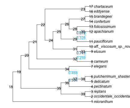
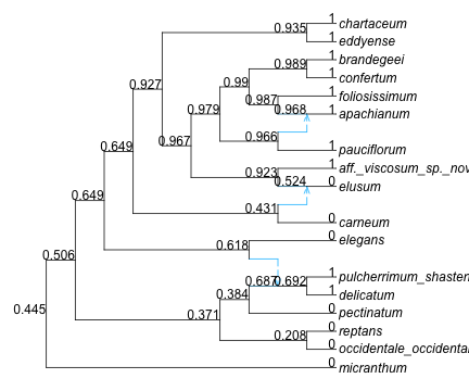
But we can map the posterior probability of state “hi” onto the network. It is important to use the network stored in the fitted object, to be assured that the node numbers match.

R"par"(mar=[0,0,0,0]);
plot(fit.net, shownodenumber=true, showgamma=true, tipoffset=0.1, xlim=[0,15]);
plot(fit.net, nodelabel=select(asr, :nodenumber, :hi), nodelabeladj=[1,-0.1],
     tipoffset=0.1, xlim=[0,15]);

effect of gene flow

What is the evidence that a trait was inherited via gene flow (along the minor hybrid edge) versus “vertically” (via the major hybrid edge)?

To answer this question, we can extract the prior probability of either option, and the posterior probabilities conditional on the data. Then, the Bayes factor to compare the 2 hypotheses, minor versus major edge (or gene flow versus vertical), can be expressed as an odds ratio: \[\mathrm{BF} = \frac{P(\mathrm{data} \mid \mathrm{minor})}{P(\mathrm{data} \mid \mathrm{mafor})} = \frac{\frac{P(\mathrm{minor} \mid \mathrm{data})}{P(\mathrm{major}\mid\mathrm{data})}}{\frac{P(\mathrm{minor})}{P(\mathrm{major})}}\,.\]

Here, let’s say we want to focus on the reticulation that is ancestral to elusum (node 33, H20). From Figure 1 (left) we see that the major (“vertical”) parent edge has γ = 0.741 = P(major) and the minor (“gene flow”) edge has γ = 0.259 = P(minor). So at this reticulation, the prior odds of the trait being inherited via gene flow is 0.259/0.741 = 0.35. Here how we may get this prior odds programmatically:

nodeH20 = net.node[findfirst(n->n.name=="H20", net.node)] # find node named H20
priorminor = getparentedgeminor(nodeH20).gamma            # γ of its minor parent
priorodds = priorminor / (1-priorminor)

0.34993311937527516

To extract the posterior odds and calculate the Bayes factor, we can do as follows, to focus on just 1 reticulation of interest and integrate out what happened at other reticulations:

postminor = exp(PhyloTraits.posterior_loghybridweight(fit, "H20"))
postodds = postminor / (1-postminor)

0.6298935555430331

That’s an increase. The Bayes factor to compare the gene flow (minor edge) versus vertical (major edge) hypotheses is then:

postodds / priorodds

1.8000398380912406

It’s above 1, so there’s evidence of inheritance via gene flow, but not very much above 1 (e.g. less than 3), so it’s equivocal evidence only.